Swim Transformer:

PatchMerging类 PatchMerging 类是 Swin Transformer 架构中用于降低特征图分辨率的层。这个过程通过合并相邻的patch来减少序列长度，同时增加通道数，以保持信息的密度。

每执行一个stage后，都会执行一个一个下采样操作，也就是PatchMerging类的前向传播。所谓的下采样操作，主要是把x切片成4个，\(x_0\)、\(x_1\)、\(x_2\)、\(x_3\)这四个是按照长宽间隔去选的：

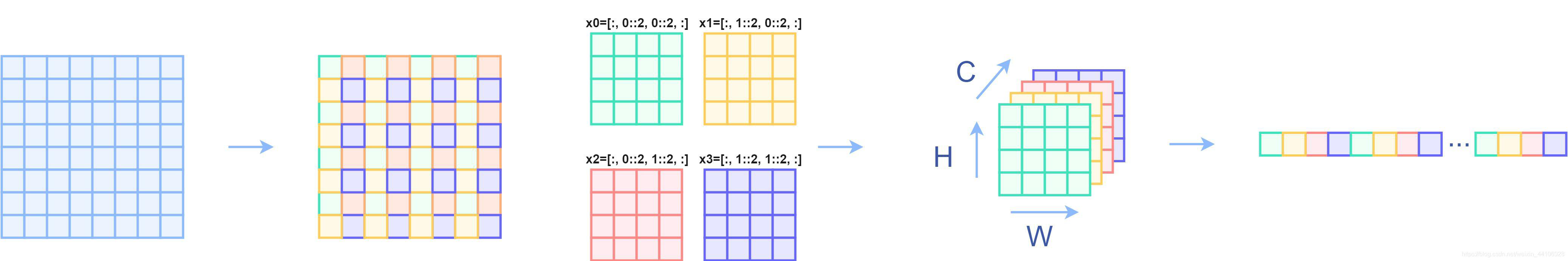
x原来是8 ∗ 8，取完后变成了4个4 ∗ 4的，再把4个做一个拼接，拼接完成后再连接一个全连接，使用全连接进行降维。

构造函数：

input_resolution ，dim ：输入特征的分辨率和通道数
reduction ，初始化一个线性变换，用于将相邻四个patch的特征合并成一个patch

前向传播：

原始输入：

torch.Size([4, 3136, 96])
2. H, W = 5656，输入特征长宽
3. B, L, C = 43136*96，batch，序列长度，特征维度
4. x： torch.Size([4, 56, 56, 96])，将输入特征重塑为四维张量，准备进行patch合并操作
5. x0： torch.Size([4, 28, 28, 96])、x1： torch.Size([4, 28, 28, 96])、x2： torch.Size([4, 28, 28, 96])、x3： torch.Size([4, 28, 28, 96])，提取四个相邻patch的特征，每个patch分别来自原始特征图的不同子区域
6. x： torch.Size([4, 28, 28, 384])，将四个patch的特征在通道维度上合并
7. x： torch.Size([4, 784, 384])，将合并后的特征图重塑，准备进行线性变换
8. x： torch.Size([4, 784, 384])，层归一化，维度不变
9. x： torch.Size([4, 784, 192])，通过线性变换降低合并后特征的维度，减少通道数

Swim Transformer code

class PatchMerging(nn.Module):
	def __init__(self, input_resolution, dim, norm_layer=nn.LayerNorm):
        super().__init__()
        self.input_resolution = input_resolution
        self.dim = dim
        self.reduction = nn.Linear(4 * dim, 2 * dim, bias=False)
        self.norm = norm_layer(4 * dim)
    def forward(self, x):
        H, W = self.input_resolution
        B, L, C = x.shape
        assert L == H * W, "input feature has wrong size"
        assert H % 2 == 0 and W % 2 == 0, f"x size ({H}*{W}) are not even."
        x = x.view(B, H, W, C)
        x0 = x[:, 0::2, 0::2, :]  # B H/2 W/2 C
        x1 = x[:, 1::2, 0::2, :]  # B H/2 W/2 C
        x2 = x[:, 0::2, 1::2, :]  # B H/2 W/2 C
        x3 = x[:, 1::2, 1::2, :]  # B H/2 W/2 C
        x = torch.cat([x0, x1, x2, x3], -1)  # B H/2 W/2 4*C
        x = x.view(B, -1, 4 * C)  # B H/2*W/2 4*C
        x = self.norm(x)
        x = self.reduction(x)
        return x

hrnet：

详情Deep High-Resolution Representation Learning for Human Pose Estimation

以下是Hrnet特征间信息交互过程，为x_fuse过程，本身并不改变各个分辨率特征的大小

fuse_layers是hrnet多个不同分辨率特征信息交互的网络，本身并不改变各个分辨率特征的大小以下为fuse_layers的构造代码：

hrnet：code

num_branches = self.num_branches
num_inchannels = self.num_inchannels
fuse_layers = []
for i in range(num_branches if self.multi_scale_output else 1):
    fuse_layer = []
    for j in range(num_branches):
        if j > i:
            fuse_layer.append(
                nn.Sequential(
                    nn.Conv2d(
                        num_inchannels[j],
                        num_inchannels[i],
                        1, 1, 0, bias=False
                    ),
                    nn.BatchNorm2d(num_inchannels[i]),
                    nn.Upsample(scale_factor=2**(j-i), mode='nearest')
                )
            )
        elif j == i:
            fuse_layer.append(None)
        else:
            conv3x3s = []
            for k in range(i-j):
                if k == i - j - 1:
                    num_outchannels_conv3x3 = num_inchannels[i]
                    conv3x3s.append(
                        nn.Sequential(
                            nn.Conv2d(
                                num_inchannels[j],
                                num_outchannels_conv3x3,
                                3, 2, 1, bias=False
                            ),
                            nn.BatchNorm2d(num_outchannels_conv3x3)
                        )
                    )
                else:
                    num_outchannels_conv3x3 = num_inchannels[j]
                    conv3x3s.append(
                        nn.Sequential(
                            nn.Conv2d(
                                num_inchannels[j],
                                num_outchannels_conv3x3,
                                3, 2, 1, bias=False
                            ),
                            nn.BatchNorm2d(num_outchannels_conv3x3),
                            nn.ReLU(True)
                        )
                    )
            fuse_layer.append(nn.Sequential(*conv3x3s))
    fuse_layers.append(nn.ModuleList(fuse_layer))

以下为fuse_layers的前向传播代码：

for i in range(len(self.fuse_layers)):
    y = x[0] if i == 0 else self.fuse_layers[i][0](x[0])
    for j in range(1, self.num_branches):
        if i == j:
            y = y + x[j]
        else:
            y = y + self.fuse_layers[i][j](x[j])
    x_fuse.append(self.relu(y))

ASPP:

Rethinking atrous convolution for semantic image segmentation

在融合的特征图上使用了ASPP模块[7]，从而可以提取出多尺度的信息。据[41]报道，全局上下文有助于收集更多的线索，如对比度差异等，用于操作检测。ASPP模块通过提取不同尺度的信息来帮助实现这方面，这样全局上下文以及更细粒度的像素级上下文信息就可用了。

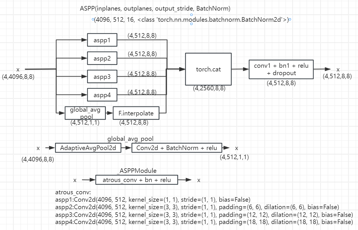
其中nn.Conv2d中的dilation参数含义如下：
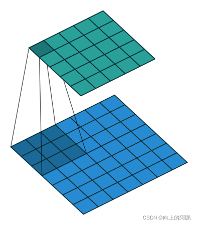
dilation = 1：

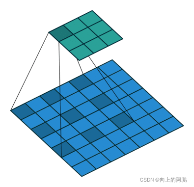
dilation=2:

ASPP code

import math
import torch
import torch.nn as nn
import torch.nn.functional as F

class _ASPPModule(nn.Module):
    def __init__(self, inplanes, planes, kernel_size, padding, dilation, BatchNorm):
        super(_ASPPModule, self).__init__()
        self.atrous_conv = nn.Conv2d(inplanes, planes, kernel_size=kernel_size,
                                            stride=1, padding=padding, dilation=dilation, bias=False)
        self.bn = BatchNorm(planes)
        self.relu = nn.ReLU()

        self._init_weight()

    def forward(self, x):
        x = self.atrous_conv(x)
        x = self.bn(x)

        return self.relu(x)

    def _init_weight(self):
        for m in self.modules():
            if isinstance(m, nn.Conv2d):
                torch.nn.init.kaiming_normal_(m.weight)
            elif isinstance(m, nn.BatchNorm2d):
                m.weight.data.fill_(1)
                m.bias.data.zero_()

class ASPP(nn.Module):
    def __init__(self, inplanes = 2048, outplanes = 512, output_stride=16, BatchNorm= nn.BatchNorm2d):
        super(ASPP, self).__init__()
        
        if output_stride == 16:
            dilations = [1, 6, 12, 18]
        elif output_stride == 8:
            dilations = [1, 12, 24, 36]
        else:
            raise NotImplementedError

        self.aspp1 = _ASPPModule(inplanes, outplanes, 1, padding=0, dilation=dilations[0], BatchNorm=BatchNorm)
        self.aspp2 = _ASPPModule(inplanes, outplanes, 3, padding=dilations[1], dilation=dilations[1], BatchNorm=BatchNorm)
        self.aspp3 = _ASPPModule(inplanes, outplanes, 3, padding=dilations[2], dilation=dilations[2], BatchNorm=BatchNorm)
        self.aspp4 = _ASPPModule(inplanes, outplanes, 3, padding=dilations[3], dilation=dilations[3], BatchNorm=BatchNorm)

        self.global_avg_pool = nn.Sequential(nn.AdaptiveAvgPool2d((1, 1)),
                                             nn.Conv2d(inplanes, outplanes, 1, stride=1, bias=False),
                                             BatchNorm(outplanes),
                                             nn.ReLU())
        self.conv1 = nn.Conv2d(outplanes*5, outplanes, 1, bias=False)
        self.bn1 = BatchNorm(outplanes)
        self.relu = nn.ReLU()
        self.dropout = nn.Dropout(0.5)
        self._init_weight()

    def forward(self, x):
        x1 = self.aspp1(x)
        x2 = self.aspp2(x)
        x3 = self.aspp3(x)
        x4 = self.aspp4(x)
        x5 = self.global_avg_pool(x)
        x5 = F.interpolate(x5, size=x4.size()[2:], mode='bilinear', align_corners=True)
        x = torch.cat((x1, x2, x3, x4, x5), dim=1)

        x = self.conv1(x)
        x = self.bn1(x)
        x = self.relu(x)

        return self.dropout(x)

    def _init_weight(self):
        for m in self.modules():
            if isinstance(m, nn.Conv2d):
                # n = m.kernel_size[0] * m.kernel_size[1] * m.out_channels
                # m.weight.data.normal_(0, math.sqrt(2. / n))
                torch.nn.init.kaiming_normal_(m.weight)
            elif isinstance(m, nn.BatchNorm2d):
                m.weight.data.fill_(1)
                m.bias.data.zero_()


def build_aspp(inplanes = 2048, outplanes = 512, output_stride=16, BatchNorm= nn.BatchNorm2d):
    return ASPP(inplanes, outplanes, output_stride, BatchNorm)

SRM 滤波器:

Rich Models for Steganalysis of Digital Images

SRM滤波器可以捕捉高频篡改痕迹，使用SRM过滤器从RGB图像中提取局部噪声特征

我们的设置中，噪声是通过像素值与仅通过内插相邻像素的值而产生的该像素值的估计之间的残差来建模的。从30个基本滤波器开始，再加上非线性运算（例如，滤波后附近输出的最大值和最小值），SRM功能将收集基本噪声特征。SRM量化并截断这些滤波器的输出，并提取附近的共现信息作为最终特征。从该过程获得的特征可以被视为局部噪声描述符。我们选择3个内核，其权重如下所示，并将其直接输入经过3通道输入训练的预训练网络中。我们将噪声流中SRM滤波器层的内核大小定义为5×5×3。SRM层的输出通道大小为3。

\[\frac {1} {4} \begin{bmatrix}0 & 0 & 0 & 0 & 0\\0 & -1 & 2 & -1 & 0\\0 & 2 & -4 & 2 & 0\\0 & -1 & 2 & -1 & 0\\0 & 0 & 0 & 0 & 0\end{bmatrix}\\\frac {1} {12} \begin{bmatrix}-1 & 2 & -2 & 2 & -1\\2 & -6 & 8 & -6 & 2\\-2 & 8 & -12 & 8 & -2\\2 & -6 & 8 & -6 & 2\\-1 & 2 & -2 & 2 & -1\end{bmatrix}\\\frac {1} {2} \begin{bmatrix}0 & 0 & 0 & 0 & 0\\0 & 0 & 0 & 0 & 0\\0 & 1 & -2 & 1 & 0\\0 & 0 & 0 & 0 & 0\\0 & 0 & 0 & 0 & 0\end{bmatrix}\]

SRM 滤波器 code 1 from CFL-Net

来自于CFL-Net

def setup_srm_weights(input_channels: int = 3, output_channel=1) -> torch.Tensor:
    """Creates the SRM kernels for noise analysis.
    note: values taken from Zhou et al., "Learning Rich Features for Image Manipulation Detection", CVPR2018
    
    Args:
        input_channels (int, optional):  Defaults to 3.
        output_channel (int, optional): Defaults to 1.
    Returns:
        torch.Tensor
    """
    srm_kernel = torch.from_numpy(
        np.array([
            [  # srm 1/2 horiz
                [0., 0., 0., 0., 0.],
                [0., 0., 0., 0., 0.],
                [0., 1., -2., 1., 0.],
                [0., 0., 0., 0., 0.],
                [0., 0., 0., 0., 0.],
            ],
            [  # srm 1/4
                [0., 0., 0., 0., 0.],
                [0., -1., 2., -1., 0.],
                [0., 2., -4., 2., 0.],
                [0., -1., 2., -1., 0.],
                [0., 0., 0., 0., 0.],
            ],
            [  # srm 1/12
                [-1., 2., -2., 2., -1.],
                [2., -6., 8., -6., 2.],
                [-2., 8., -12., 8., -2.],
                [2., -6., 8., -6., 2.],
                [-1., 2., -2., 2., -1.],
            ]
        ])).float()
    srm_kernel[0] /= 2
    srm_kernel[1] /= 4
    srm_kernel[2] /= 12
    return srm_kernel.view(3, 1, 5, 5).repeat(output_channel, input_channels, 1, 1)
    
def setup_srm_layer(input_channels: int = 3, output_channel=None) -> torch.nn.Module:
    """Creates a SRM convolution layer for noise analysis.
    Args:
        input_channels (int, optional): [description]. Defaults to 3.
        output_channel ([type], optional): [description]. Defaults to None.
    Returns:
        torch.nn.Module: [description]
    """
    if output_channel == None:
        weights = setup_srm_weights(input_channels)
        conv = torch.nn.Conv2d(input_channels, out_channels=3, kernel_size=5, stride=1, padding=2, bias=False)
    else:
        weights = setup_srm_weights(input_channels, output_channel)
        conv = torch.nn.Conv2d(input_channels,
                               out_channels=output_channel,
                               kernel_size=5,
                               stride=1,
                               padding=2,
                               bias=False)
    with torch.no_grad():
        conv.weight = torch.nn.Parameter(weights, requires_grad=False)
    return conv

SRM 滤波器 code 2 from Towards Generic Image Manipulation Detection with Weakly-Supervised Self-Consistency Learning

来自于Towards Generic Image Manipulation Detection with Weakly-Supervised Self-Consistency Learning

SRM滤波器[14，66]使用预定义的核来学习中心像素的相邻像素之间不同类型的噪声残差，然后进行线性或非线性的最大/最小运算。

import numpy as np
import torch
import torch.nn as nn


class SRMConv2d(nn.Module):
    def __init__(self, stride: int = 1, padding: int = 2, clip: float = 2):
        super().__init__()
        self.stride = stride
        self.padding = padding
        self.clip = clip
        self.conv = self._get_srm_filter()

    def _get_srm_filter(self):
        filter1 = [
            [0, 0, 0, 0, 0],
            [0, -1, 2, -1, 0],
            [0, 2, -4, 2, 0],
            [0, -1, 2, -1, 0],
            [0, 0, 0, 0, 0],
        ]
        filter2 = [
            [-1, 2, -2, 2, -1],
            [2, -6, 8, -6, 2],
            [-2, 8, -12, 8, -2],
            [2, -6, 8, -6, 2],
            [-1, 2, -2, 2, -1],
        ]
        filter3 = [
            [0, 0, 0, 0, 0],
            [0, 0, 0, 0, 0],
            [0, 1, -2, 1, 0],
            [0, 0, 0, 0, 0],
            [0, 0, 0, 0, 0],
        ]
        q = [4.0, 12.0, 2.0]
        filter1 = np.asarray(filter1, dtype=float) / q[0]
        filter2 = np.asarray(filter2, dtype=float) / q[1]
        filter3 = np.asarray(filter3, dtype=float) / q[2]
        filters = [
            [filter1, filter1, filter1],
            [filter2, filter2, filter2],
            [filter3, filter3, filter3],
        ]
        filters = torch.tensor(filters).float()
        conv2d = nn.Conv2d(
            3,
            3,
            kernel_size=5,
            stride=self.stride,
            padding=self.padding,
            padding_mode="zeros",
        )
        conv2d.weight = nn.Parameter(filters, requires_grad=False)
        conv2d.bias = nn.Parameter(torch.zeros_like(conv2d.bias), requires_grad=False)
        return conv2d

    def forward(self, x):
        x = self.conv(x)
        if self.clip != 0.0:
            x = x.clamp(-self.clip, self.clip)
        return x


if __name__ == "__main__":
    srm = SRMConv2d()
    x = torch.rand((63, 3, 64, 64))
    x = srm(x)

BayarConv:

Belhassen Bayar and Matthew C Stamm. Constrained convolutional neural networks: A new approach towards general purpose image manipulation detection

Bayar卷积滤波器[2]通过使用可学习权重来改进SRM滤波器，约束条件是相邻像素的加权和等于中心像素的权重的负。

BayarConv code 1 from Towards Generic Image Manipulation Detection with Weakly-Supervised Self-Consistency Learning

来自于Towards Generic Image Manipulation Detection with Weakly-Supervised Self-Consistency Learning

import torch
import torch.nn as nn
from einops import rearrange


class BayarConv2d(nn.Module):
    def __init__(
        self,
        in_channles: int,
        out_channels: int,
        kernel_size: int = 5,
        stride: int = 1,
        padding: int = 0,
        magnitude: float = 1.0,
    ):
        super().__init__()
        assert kernel_size > 1, "Bayar conv kernel size must be greater than 1"

        self.in_channels = in_channles
        self.out_channels = out_channels
        self.kernel_size = kernel_size
        self.stride = stride
        self.padding = padding
        self.magnitude = magnitude

        self.center_weight = nn.Parameter(
            torch.ones(self.in_channels, self.out_channels, 1) * -1.0 * magnitude,
            requires_grad=False,
        )
        self.kernel_weight = nn.Parameter(
            torch.rand((self.in_channels, self.out_channels, kernel_size**2 - 1)),
            requires_grad=True,
        )

    def _constraint_weight(self):
        self.kernel_weight.data = self.kernel_weight.permute(2, 0, 1)
        self.kernel_weight.data = torch.div(
            self.kernel_weight.data, self.kernel_weight.data.sum(0)
        )
        self.kernel_weight.data = self.kernel_weight.permute(1, 2, 0) * self.magnitude
        center_idx = self.kernel_size**2 // 2
        full_kernel = torch.cat(
            [
                self.kernel_weight[:, :, :center_idx],
                self.center_weight,
                self.kernel_weight[:, :, center_idx:],
            ],
            dim=2,
        )
        full_kernel = rearrange(
            full_kernel, "ci co (kw kh) -> ci co kw kh", kw=self.kernel_size
        )
        return full_kernel

    def forward(self, x):
        x = nn.functional.conv2d(
            x, self._constraint_weight(), stride=self.stride, padding=self.padding
        )
        return x


if __name__ == "__main__":
    device = "cuda"
    bayer_conv2d = BayarConv2d(3, 3, 3, magnitude=1).to(device)
    bayer_conv2d._constraint_weight()
    i = torch.rand(16, 3, 16, 16).to(device)
    o = bayer_conv2d(i)

% 读取图像
grayImage = imread('image.jpg');

% 检查图像是否为灰度图像，如果不是，转换为灰度图像
if size(grayImage, 3) == 3
    grayImage = rgb2gray(grayImage);
end

% 显示灰度图像
imshow(grayImage);
title('显示灰度图像');

% 保存灰度图像
imwrite(grayImage, 'grayImage.png');

CBAM: Convolutional Block Attention Module:

本文出自2018ECCV会议

论文地址：https://arxiv.org/abs/1807.06521

一、计算机视觉中的注意力机制

在计算机视觉中能够能够把注意力聚集在图像重要区域而丢弃掉不相关的方法被称作是注意力机制(Attention Mechanisms)。在人类视觉大脑皮层中，使用注意力机制能够更快捷和高效地分析复杂场景信息。这种机制后来被研究人员引入到计算机视觉中来提高性能。注意力机制可以看做是对图像输入重要信息的动态选择过程，这个过程是由对于特征自适应权重实现的。注意力机制极大提升了很多计算机视觉任务性能水平，比如在分类，目标检测，语义分割，人脸识别，动作识别，小样本检测，医疗影像处理，图像生成，姿态估计，超分辨率，3D视觉以及多模态中等任务中发挥着重要作用。
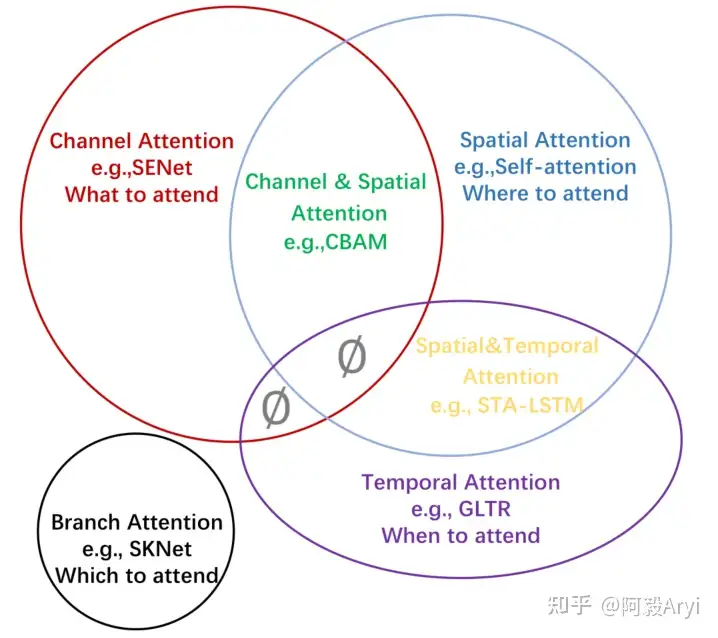
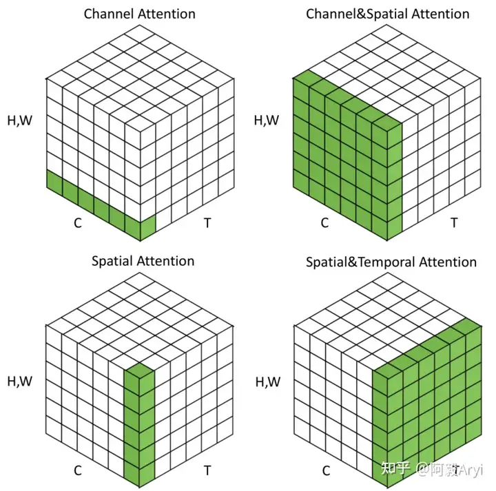
一般来说，注意力机制通常被分为以下基本四大类：

通道注意力 Channel Attention，告诉网络 what to pay attention to
空间注意力机制 Spatial Attention，告诉网络 where to pay attention to
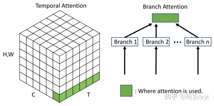
时间注意力机制 Temporal Attention，告诉网络 when to pay attention
分支注意力机制 Branch Attention，告诉网络 which to pay attention to

最后还有两种混合注意力机制：

通道&空间注意力机制 和 空间&时间注意力机制。

不同种类的注意力机制在不同的视觉任务中的效果是不同的。

二、CBAM: Convolutional Block Attention Module

本文提出的Convolutional Block Attention Module(CBAM)就是上面所提到的两种混合注意力中通道&空间注意力的一种。在给定一张特征图，CBAM模块能够序列化地在通道和空间两个维度上产生注意力特征图信息，然后两种特征图信息在与之前原输入特征图进行相乘进行自适应特征修正，产生最后的特征图。CBAM是一种轻量级的模块，可以嵌入到任何主干网络中以提高性能。

1.设计启发

CNN网络由于其强大的特征表示能力极大地提高了计算机视觉任务的水平，为了进一步增强这种特征表达能力，研究者在三个主要方面对其进行了更深入地研究，分别是网络的深度，网络的宽度，网络的维度。
在深度研究层面，像是我们熟知的最早先的网络LeNet，到深度逐渐加深的采用1x1卷积和3x3卷积不断堆叠的VGGNet，再到采用了残差设计的ResNet，证实了网络可以堆叠到几百层甚至上千层。GoogLeNet设计了Inception模块可以对网络的宽度进行研究并证明了其效果。Xception和ResNeXt提出了网络另一个维度Cardinality，证实了这个维度不仅可以节约大量参数而且展示出了比深度和宽度有更强特征表达能力的效果。
所以在除了在以上维度对CNN的特征表达能力进行研究之外，作者对网络结构的另外一个层面进行了探索，那就是注意力机制。早前的注意力机制研究已经进行的如火如荼了。注意力机制的主要目的就是：聚焦图像的重要特征，抑制不必要的区域响应，通过在对通道维度和空间维度组合分析研究，提出了CBAM模块，并证实了网络的性能的提升来自于精确的注意力机制和对无相关噪声信息的抑制。

2.CBAM总体流程

对于网络主干生成的特征图： \[F\in R^{C\times H\times W}\] CBAM分别产生1D通道注意力特征图、2D空间注意力特征图： \[M_c\in R^{C\times 1\times 1}\\M_s\in R^{1\times H\times W}\] 这个过程我们可以描述为以下公式： \[F^{'}=M_{c}(F)\otimes F\\F^{''}=M_{s}(F^{'})\otimes F^{'}\] \(\otimes\)表示元素级相乘，中间采用广播机制进行维度变换和匹配。

3.Channel Attention Module

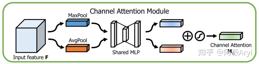
先看通道注意力机制，通过特征内部之间的关系来通道注意力机制。特征图的每个通道都用来被视作一个特征检测器，所以通道特征聚焦的是图像中有用的信息是"什么"（what）。
为了更高效地计算通道注意力特征，要做的就是压缩特征图的空间维度，之前采用的是平均池化方法，这个方法可以学习到目标物体的程度信息，作者这里研究了最大池化也能够学习到物体的判别性特征。所以在通道注意力模块同时采用了这两种方法，在后面的实验中也证实了，同时使用两种方法要比单独使用一种方法效果要好。
在经过这种方法之后产生了两种不同的空间上下文信息：\(F_{avg}^c\) 和 \(F_{max}^c\) 分别代表平均池化特征和最大池化特征。
然后再将该特征送入到一个共享的多层感知机(MLP)网络中产生最终的通道注意力特征图 \(M_c\in R^{C\times 1\times 1}\)
为了降低计算参数，在MLP中采用了一个降维系数r， \(M_c\in R^{C/r\times 1\times 1}\)
综上通道注意力计算公式总结为： \[\begin{gathered}M_{c}(F) =\sigma(MLP(AvgPool(F))+MLP(MaxPool(F))) \\=\sigma(W_{1}(W_{0}(F_{avg}^{c}))+W_{1}(W_{0}(F_{max}^{c}))) \end{gathered}\]

4.Spatial Attention Module

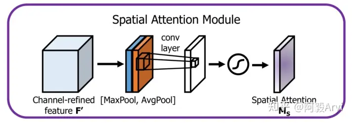
通过对特征图空间内部的关系来产生空间注意力特征图。不同于通道注意力，空间注意力聚焦于特征图上的有效信息在"哪里"（where）。为了计算空间注意力，首先在通道维度平均池化和最大池化，然后将他们产生的特征图进行拼接起来（concat）。然后在拼接后的特征图上，使用卷积操作来产生最终的空间注意力特征图： \[M_s(F)\in R^{1\times H\times W}\] 同上，在通道维度使用两种池化方法产生2D特征图：

\[F_{avg}^c \in R^{1\times H\times W}\\F_{max}^c \in R^{1\times H\times W}\] 最终这个过程的公式如下： \[\begin{aligned}M_{s}(F)& =\sigma(f^{7\times7}([AvgPool(F);MaxPool(F)])) \\&=\sigma(f^{7\times7}(F_{avg}^{s};F_{max}^{s}))\end{aligned}\]

三.代码实现

经过上面的分析，我们可以看到CBAM主要包括两个部分，Channel Attention Module 和 Spatial Attention Module，其实际的代码也是非常通俗易懂。
下面是pytorch版本的代码。

#通道注意力
class ChannelAttention(nn.Module):
    def __init__(self, in_planes, ratio=16):
        super(ChannelAttention, self).__init__()
        self.avg_pool = nn.AdaptiveAvgPool2d(1)
        self.max_pool = nn.AdaptiveMaxPool2d(1)
        
        #MLP  除以16是降维系数
        self.fc1   = nn.Conv2d(in_planes, in_planes // 16, 1, bias=False) #kernel_size=1
        self.relu1 = nn.ReLU()
        self.fc2   = nn.Conv2d(in_planes // 16, in_planes, 1, bias=False)

        self.sigmoid = nn.Sigmoid()

    def forward(self, x):
        avg_out = self.fc2(self.relu1(self.fc1(self.avg_pool(x))))
        max_out = self.fc2(self.relu1(self.fc1(self.max_pool(x))))
        #结果相加
        out = avg_out + max_out
        return self.sigmoid(out)

#空间注意力
class SpatialAttention(nn.Module):
    def __init__(self, kernel_size=7):
        super(SpatialAttention, self).__init__()
        #声明卷积核为 3 或 7
        assert kernel_size in (3, 7), 'kernel size must be 3 or 7'
        #进行相应的same padding填充
        padding = 3 if kernel_size == 7 else 1

        self.conv1 = nn.Conv2d(2, 1, kernel_size, padding=padding, bias=False)
        self.sigmoid = nn.Sigmoid()

    def forward(self, x):
        avg_out = torch.mean(x, dim=1, keepdim=True)  #平均池化
        max_out, _ = torch.max(x, dim=1, keepdim=True) #最大池化
        #拼接操作
        x = torch.cat([avg_out, max_out], dim=1)
        x = self.conv1(x) #7x7卷积填充为3，输入通道为2，输出通道为1
        return self.sigmoid(x)